Supervised Machine Learning - Classification Learning

In supervised learning, the model use labelled dataset to predict the output. Here, labelled dataset means a dataset contains both input and output values.

In machine learning, few terminologies are important to know and I will use these terminologies interchangeably throughout the blog.

Classification

Classification is one type of supervised learning, in which the classification models are used to find which class the new data belongs to based on two or more independent variables.

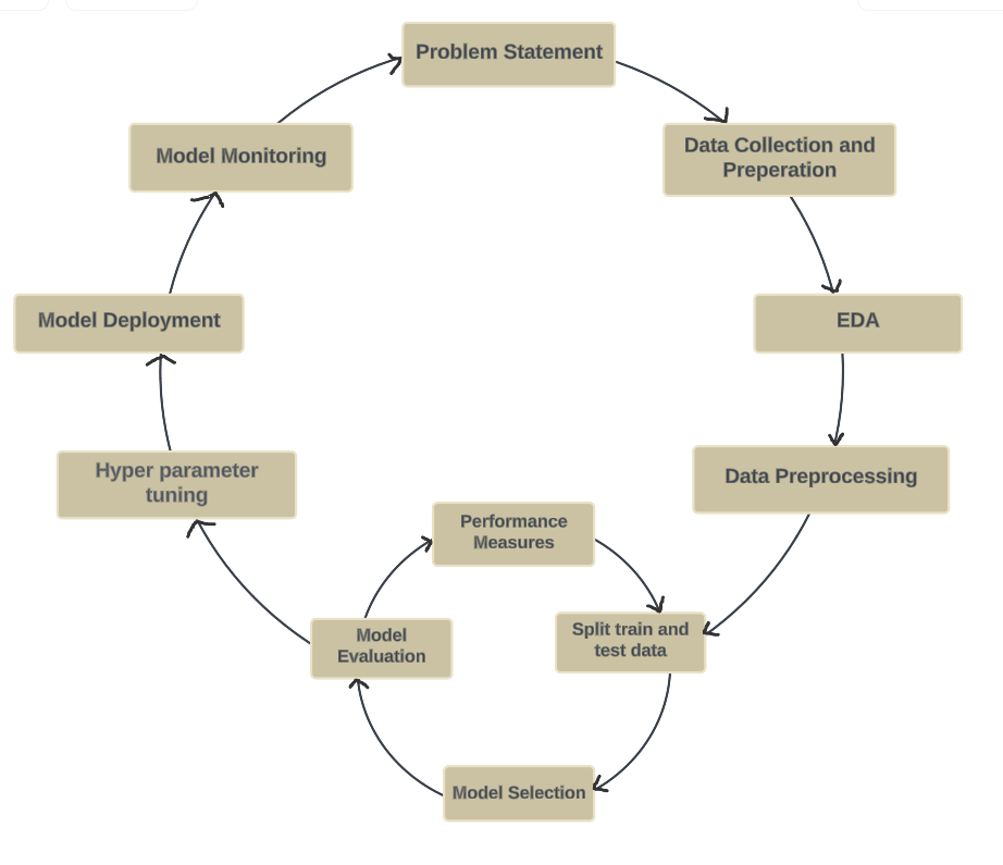
Workflow of Supervised Learning

For every model in supervised learning follows same steps of training and validating a model.

1. Data Collection

I took dataset from 'Kaggle' and for the classification models I used 'Employee Attrition Prediction' dataset.

Firstly, import necessary libraries to load the dataset

# pandas - used for manipulation and analysis library
import pandas as pd
# numpy - supports large, multi-dimensional arrays and matrices, and high-level mathematical functions.
import numpy as np

# Load the dataset using 'read_csv'
employee_data = pd.read_csv('.../kaggle/employee-attritiion.csv')

# To see first 5 rows of data
employee_data.head()

# To know size of our data
employee_data.shape() # (74498, 24)

2. Data Preperation

In this step, we will find if the data has any missing values, duplicate values or errors.

Data Cleaning: Handle missing values, remove duplicates, and correct errors.

# find missing values - see if data has any NaN values
employee_data.isnull().sum()

# output - 
# Employee ID  0
# Age          0
# Gender       0 etc...

# find duplicate values - see if values are repeated
employee_data.duplicated()
# or
employee_data[employee_data.duplicated()]
# returns all duplicated rows

# In our case there are no duplicates and missing values

3. Exploratory Data Analysis (EDA)

Now its time to visualize the data using matplotlib and seaborn libraries in python. This step helps us to analyze the data to understand patterns, relationships, and insights.

Techniques: Visualizations (histograms, scatter plots), summary statistics, correlation analysis.

# let's find unique values in our dataset
for col in employee_data.columns:
    print(f'{col}: ', employee_data[col].unique())
    
# Employee ID:  [ 8410 64756 30257 ... 12409  9554 73042]
# Age:  [31 59 24 ... 22 32]
# Gender:  ['Male' 'Female']
# Years at Company:  [19 15 ... 50 51]
# Job Role:  ['Education' 'Media' 'Healthcare' 'Technology' 'Finance']
# Monthly Income:  [ 5390  5534  8159 ... 11854 11558 12651]
# Work-Life Balance:  ['Excellent' 'Poor' 'Good' 'Fair']
# Job Satisfaction:  ['Medium' 'High' 'Very High' 'Low']
# Performance Rating:  ['Average' 'Low' 'High' 'Below Average']
# Number of Promotions:  [2 3 0 1 4]
# Overtime:  ['No' 'Yes']
# Distance from Home:  [22 21 .... 66]
# Education Level:  ['Associate Degree' 'Master’s Degree' 'Bachelor’s Degree' 'High School'
 'PhD']
# Marital Status:  ['Married' 'Divorced' 'Single']
# Number of Dependents:  [0 3 2 4 1 5 6]
# Job Level:  ['Mid' 'Senior' 'Entry']
# Company Size:  ['Medium' 'Small' 'Large']
# Company Tenure:  [ 89  21  .... 126 128]
# Remote Work:  ['No' 'Yes']
# Leadership Opportunities:  ['No' 'Yes']
# Innovation Opportunities:  ['No' 'Yes']
# Company Reputation:  ['Excellent' 'Fair' 'Poor' 'Good']
# Employee Recognition:  ['Medium' 'Low' 'High' 'Very High']
# Attrition:  ['Stayed' 'Left']

From this we can see that we have both numerical values (Age, Years at company, Monthly income etc..) and categorical values (work-life balance, performance rating, gender etc.. ). This means that we have to convert categorical values to numerical encoding in preprocessing step (which is in next step).

# Let's define out input features and output target variables

X = employee_data.drop(['Employee ID', 'Attrition'])
y = employee_data['Attrition']

X.shape # (74498, 22)
y.shape # (74498,)

4. Data Preprocessing

In this step we do data transformation and feature engineering on datasets.

• Data Transformation: Normalize or standardize features, encode categorical variables.
• Feature Engineering: Create new features from existing data to improve model performance.

Let's transform our categorical data to numerical values using ordinal encoder, label encoder and one-hot encoder.

a. Data encoding:

• Ordinal encoder: Converts categorical features into integer values based on their rank or order. Example - [ 'low', medium', 'high' ]
• Label encoder: Converts categorical text data into model-understandable numerical data without an inherent order. Mostly used for target variables
• One-hot encoder: Converts categorical variables into a set of binary (0 or 1) columns. Example: 'health-care': 001, 'IT': 010, 'education': 100

from sklearn.preprocessing import OrdinalEncoder

# ordinal encoding for features
columns_to_encode = ['Work-Life Balance', 'Job Satisfaction', 'Performance Rating', 'Education Level', 'Job Level', 'Company Size', 'Company Reputation', 'Employee Recognition']

categories=[
    ['Poor', 'Fair', 'Good', 'Excellent'], # Work-Life Balance
    ['Low', 'Medium', 'High', 'Very High'], # Job Satisfaction
    ['Low', 'Below Average', 'Average', 'High'], # Performance Rating
    ["High School", "Bachelor’s Degree", "Master’s Degree", "Associate Degree", "PhD"], # Education Level
    ['Entry', 'Mid', 'Senior'], # Job Level
    ['Small', 'Medium', 'Large'], # Company Size
    ['Poor', 'Fair', 'Good', 'Excellent'], # Company Reputation
    ['Low', 'Medium', 'High', 'Very High'], # Employee Recognition
]

oe = OrdinalEncoder(categories=categories)

X[columns_to_encode] = oe.fit_transform(X[columns_to_encode])

# define numerical encoder
emp_bool_map = ['Overtime', 'Remote Work', 'Leadership Opportunities', 'Innovation Opportunities']

for col in emp_bool_map:
    X[col] = X[col].map({'No': 0, 'Yes': 1})

# -----------------------------------------------
# label encoding for target values
y = y.map({'Stayed': 0, 'Left': 1})

# -----------------------------------------------
# one-hot encoding
X = pd.get_dummies(X)
X.head()

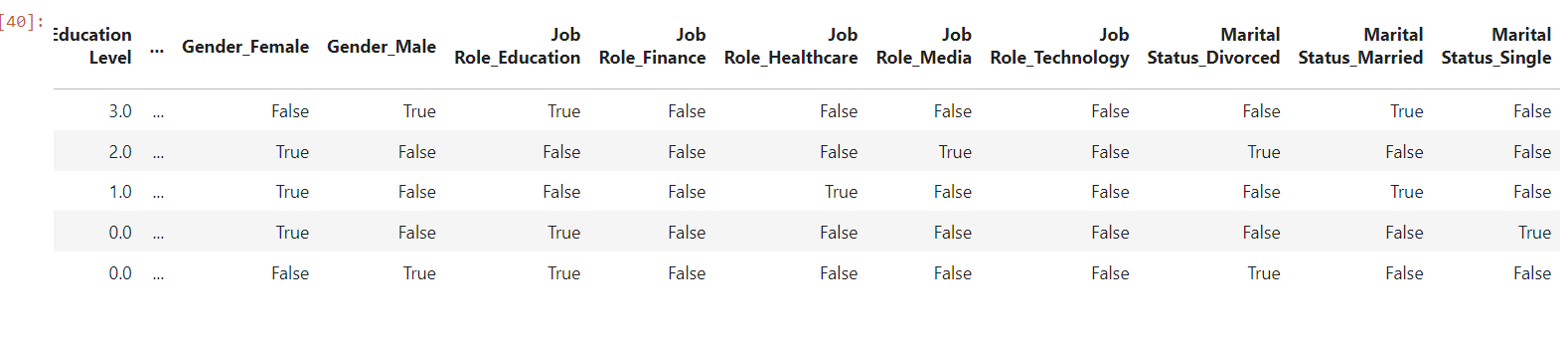
Did you see that gender, job-role and marital status are break down into gender_male, gender_female, job_role_healthcare etc... This is due to one-hot encoding, which used when it does not have any impact to output but we want to include it in features.

b. Data scaling and normalization:

Once data is encoded it is time to scale the features into single unit by making it a mean of '0' and a standard deviation of '1'. It is used when features have different units or scales.

step-1: Split the X and y into training set and test set.

step-2: Apply scaling to train and test datasets.

# first split the data into train and test sets

from sklearn.preprocessing import StandardScaler
from sklearn.model_selection import train_test_split

X_train, X_test, y_train, y_test = train_test_split(X_scaled, y, test_size=0.2, random_state=42)

X_train.shape # (59598, 29)
X_test.shape # (14900, 29)

# scaling the features
scaler = StandardScaler()
X_train = scaler.fit_transform(X_train)
X_test = scaler.transform(X_test)

5. Model Selection

One has to experiment on different models and check its performance with test data. The model with high accuracy will predict outcome better.

Logistic Regression

Despite its name, logistic regression is used for binary classification tasks.

• It predicts the probability of an instance belonging to a particular class. In other words, it predicts which class a new data will belongs to based on outcome of probability. 
• Similar like linear regression, instead it is used when target variable is not a number but categorical type such as green/blue, cat/dog etc.
• This algorithm use sigmoid function, which is a mathematical function used to map the predicted values to probabilities. It maps any real value into another value within a range of 0 and 1.

# Logistic regression

from sklearn.linear_model import LogisticRegression
from sklearn.metrics import accuracy_score, confusion_matrix, classification_report

lr = LogisticRegression()
model_lr = lr.fit(X_train, y_train)

# predict outcome with test data
y_pred_lr = model_lr.predict(X_test)

# compare the performance of our test-data with new predicted values
accuracy = accuracy_score(y_test, y_pred_lr)
confusion_mat = confusion_matrix(y_test, y_pred_lr)
classification = classification_report(y_test, y_pred_lr)

print('Accuracy: ', accuracy*100)
print(classification)
print(confusion_mat)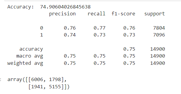

Performance Metrics:

• Accuracy: The overall accuracy of the model is 74.91% appx, which means that the model correctly predicts the target variable (attrition) approximately 75% of the time.
• Precision:
  • Precision for Class 0 (Stayed): 0.76Precision indicates the percentage of correctly predicted positives out of the total predicted positives for this class.For class 0, 76% of the instances predicted as "Stayed" are actually "Stayed".
  • Precision for Class 1 (Left): 0.74For class 1, 74% of the instances predicted as "Left" are actually "Left
• Recall:
  • Indicates the percentage of correctly predicted positives out of the actual positives for this class.
  • For class 0, 77% of the instances that are actually "Stayed" are correctly predicted by the model.
  • Recall for Class 1 (Left): 0.73For class 1, 73% of the instances that are actually "Left" are correctly predicted by the model.
• F1-Score:
  • The F1-score is the harmonic mean of precision and recall, providing a single metric that balances both concerns.
  • F1-Score for Class 0 (Stayed): 0.76
  • F1-Score for Class 1 (Left): 0.73
• Support:
  • Support for Class 0 (Stayed): 7804The number of actual occurrences of the class in the test set.
  • Support for Class 1 (Left): 7096
• Confusion Matrix:
  • True Positives (TP) for Class 0: 6006 (correctly predicted "Stayed")
  • False Positives (FP) for Class 0: 1798 (incorrectly predicted as "Stayed" but actually "Left")
  • False Negatives (FN) for Class 1: 1941 (incorrectly predicted as "Left" but actually "Stayed")
  • True Positives (TP) for Class 1: 5155 (correctly predicted "Left")

Summary:

• The model has a balanced precision and recall for both classes, indicating it can predict both "Stayed" and "Left" with reasonable accuracy.
• The model performs slightly better in predicting employees who stayed (Class 0) than those who left (Class 1), but the difference is not large.
• Given the accuracy and the balanced precision and recall scores, this logistic regression model performs reasonably well for predicting employee attrition.

6. Model Deployement

After predicting our logistic model with test set and observing its performance metrics, lets use our model in web development. This can be achieved by using 'pickle' library.

Pickle library: Used for serializing and deserializing Python objects. This is useful for saving the state of an object to a file or sending it over a network, and then later reconstructing the object.

# To use our model in web development, lets serialize our model into file.

import pickle
with open("my_model.pkl", "wb") as f:
    pickle.dump((model_lr, scaler, X.columns.to_list()), f)

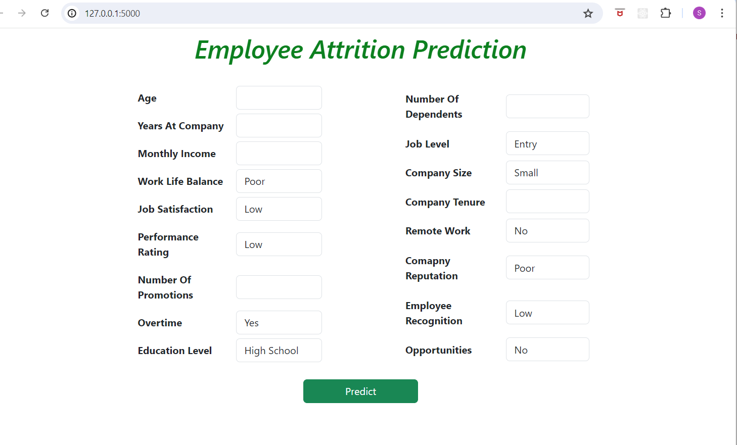
Frontend

Used 'Flask' for creating both frontend application and backend for using our model. There are other ways to use our model using APIs, by creating an API of our model and then calling this API to frontend application of different language like JavaScript, C# etc.

Folder Structure of my project in 'Flask':

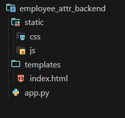
In index.html, I created a form consisting of - Age, Years at Company, Monthly Income, Work-Life Balance, Job Satisfaction etc.. features which is same as the features I gave in model.

Backend

Create a file "app.py", and follow the code below:

import os
import pickle
import numpy as np
import pandas as pd
from flask import Flask, request, jsonify, render_template
from flask_cors import CORS

# sart flask app
app = Flask(__name__)

# Cors - to remove cross-origin error request
CORS(app)

# load the model, scaler and ordinal-encoder
if os.path.isfile("D:/machine learning/basics/my_model_lr.pkl"):
    with open("D:/machine learning/basics/my_model_lr.pkl", "rb") as f:
        model_lr, scaler, OrdinalEncoder = pickle.load(f)
else:
    raise FileNotFoundError

# data pre-processing for new data - similar like we gave in "training our model".
columns_to_encode = ['Work-Life Balance', 'Job Satisfaction', 'Performance Rating', 'Education Level', 'Job Level', 'Company Size', 'Company Reputation', 'Employee Recognition']

categories=[
    ['Poor', 'Fair', 'Good', 'Excellent'],
    ['Low', 'Medium', 'High', 'Very High'],
    ['Low', 'Below Average', 'Average', 'High'],
    ["High School", "Bachelor’s Degree", "Master’s Degree", "Associate Degree", "PhD"],
    ['Entry', 'Mid', 'Senior'],
    ['Small', 'Medium', 'Large'],
    ['Poor', 'Fair', 'Good', 'Excellent'],
    ['Low', 'Medium', 'High', 'Very High'],
]

# define numerical encoder...
emp_bool_map = ['Overtime', 'Remote Work', 'Opportunities']

# ------------------
# home page
@app.route('/')
def index():
    return render_template('index.html')

# -----------------
# start route
@app.route('/predict', methods=['POST'])
def predict():
    # get json data
    data = request.get_json()

    # convert requested data to dataframe for further analysis
    X_new = pd.DataFrame([data])

    # apply encoding
    oe = OrdinalEncoder(categories=categories)
    X_new[columns_to_encode] = oe.fit_transform(X_new[columns_to_encode]).astype('int')

    for name in emp_bool_map:
        X_new[name] = X_new[name].map({'No': 0, 'Yes': 1})

    # Define the function to map income ranges to ordinal values
    def map_monthly_income(income):
        if 1200 <= income <= 5000:
            return 0
        elif 5001 <= income <= 10000:
            return 1
        elif 10001 <= income <= 15000:
            return 2
        elif 15001 <= income <= 20000:
            return 3
        elif income >= 20001:
            return 4
        else:
            return -1  # Handle any unexpected values

    X_new['Monthly Income'] = X_new['Monthly Income'].apply(map_monthly_income)

    # use standard scaler to scale the features
    features = scaler.transform(X_new)
    
    # predict the output
    y_pred = model_lr.predict(features)

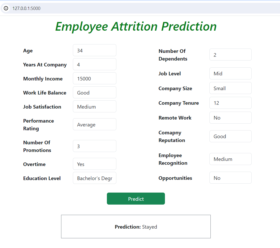
    prediction = "Left" if y_pred[0] == 1 else "Stayed"

    return jsonify({'prediction': prediction})

if __name__=='__main__':
    app.run(debug=True)

Here is the outcome of the employee attrition application

For further analysis we can do feature engineering and hyper parameter tuning.

• By calculating difference between "years at company" and "company tenure", so that a new feature "years at previous company" gives us insights about behaviour of employee - how frequently he jumps from one company to other.
• Also data is looking inconsistent in "company tenure" one can remove inconsistent data or replace it with NaN or 0 value.
• Hyper-tuning used to optimize the model’s performance by tuning its hyperparameters. Techniques like grid search, random search and Bayesian optimization are used for optimization.

To get the frontend code, follow this link Employee Attrition Prediction Applicaion

Thank you for reading my article and follow techiescamp-blog to know more about MLOPS.